Confusion Matrix for Experiment Readouts
A confusion matrix turns binary outcomes into countable diagnostics. In experiment and measurement workflows, it helps separate model quality from class balance:
- True positive (TP): predicted positive and observed positive
- False positive (FP): predicted positive and observed negative
- False negative (FN): predicted negative and observed positive
- True negative (TN): predicted negative and observed negative
2x2 count table
For binary outcomes, keep counts in a standard layout with marginals:
| Observed \ Predicted | + | - | Row total |
|---|---|---|---|
| + | TP | FN | TP + FN |
| - | FP | TN | FP + TN |
| Column total | TP + FP | FN + TN | N |
From this table:
\[ \begin{aligned} \text{TPR} &= \text{sensitivity} = \text{recall} = \frac{TP}{TP + FN}, \\ \text{TNR} &= \text{specificity} = \frac{TN}{TN + FP}, \\ \text{PPV} &= \text{precision} = \frac{TP}{TP + FP}, \\ \text{NPV} &= \frac{TN}{TN + FN}, \\ \text{accuracy} &= \frac{TP + TN}{TP + FP + FN + TN}, \\ F_1 &= \frac{2 \cdot \text{precision} \cdot \text{recall}}{\text{precision} + \text{recall}}. \end{aligned} \]
Standard deviation under model assumptions
Rate uncertainty depends on the data-generating assumption behind each metric denominator.
Assumption A: independent Bernoulli trials (binomial model)
For a rate \(\hat p = x/n\) (for example recall with \(x=TP\), \(n=TP+FN\)),
\[ \operatorname{SD}(\hat p) = \sqrt{\frac{\hat p(1-\hat p)}{n}}. \]
Derivation of the SD equation
Let \(Y_i \in \{0,1\}\) indicate whether trial \(i\) is a success, with \(\Pr(Y_i=1)=p\), and assume \(Y_1,\dots,Y_n\) are independent and identically distributed. Define the sample proportion:
\[ \hat p = \frac{1}{n}\sum_{i=1}^{n} Y_i. \]
Because a Bernoulli variable satisfies \(\operatorname{Var}(Y_i)=p(1-p)\),
\[ \operatorname{Var}(\hat p) = \operatorname{Var}\!\left(\frac{1}{n}\sum_{i=1}^{n} Y_i\right) = \frac{1}{n^2}\sum_{i=1}^{n}\operatorname{Var}(Y_i) = \frac{1}{n^2}\cdot n\,p(1-p) = \frac{p(1-p)}{n}. \]
So the standard deviation is
\[ \operatorname{SD}(\hat p)=\sqrt{\operatorname{Var}(\hat p)} = \sqrt{\frac{p(1-p)}{n}}. \]
In practice, \(p\) is unknown, so replace it with \(\hat p\) to get the plug-in estimate used above:
\[ \widehat{\operatorname{SD}}(\hat p) = \sqrt{\frac{\hat p(1-\hat p)}{n}}. \]
This is the default planning approximation for recall, precision, specificity, and accuracy when outcomes are independent inside each denominator group.
Assumption B: large-sample normal approximation
If \(n\hat p\) and \(n(1-\hat p)\) are both reasonably large, use
\[ \hat p \pm z_{\alpha/2}\,\operatorname{SD}(\hat p) \]
as an approximate confidence interval. Typical multipliers are:
- \(z \approx 1\) for about 68% coverage
- \(z \approx 1.96\) for about 95% coverage
- \(z \approx 3\) for conservative 3-SD screening
Assumption C: overdispersed Bernoulli (beta-binomial style)
When repeated measurements are correlated (batch effects, instrument drift, cohort structure), inflate variance with a dispersion factor \(\phi \ge 1\):
\[ \operatorname{SD}_{\text{over}}(\hat p) = \sqrt{\phi}\,\operatorname{SD}(\hat p). \]
A beta-binomial model makes that inflation explicit:
\[ X \mid θ \sim \operatorname{Binomial}(n, θ), \qquad θ \sim \operatorname{Beta}(α, β), \qquad \hat p = \frac{X}{n}. \]
If \(\mu = \mathbb{E}[θ]\), then
\[ \mathbb{E}[\hat p] = \mu, \qquad \operatorname{Var}(\hat p) = \frac{\mu(1-\mu)}{n}\,\Bigl[1 + (n-1)\rho\Bigr], \]
where \(\rho = 1/(α + β + 1)\) is the intra-class correlation. In the notation above, \(\phi = 1 + (n-1)\rho\).
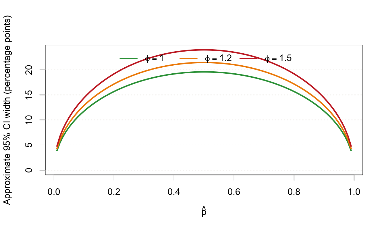
Before introducing \(\phi\), the CI width is fixed by \(\hat p\) and \(n\) through the binomial standard deviation. After introducing \(\phi\), the same \(\hat p\) can produce a wider interval because the width is multiplied by \(\sqrt{\phi}\).
Use this when empirical residuals are wider than binomial expectations.
Example matrix
| Observed Predicted | Predicted + | Predicted - | Row total |
|---|---|---|---|
| + | 84 | 24 | 108 |
| - | 16 | 176 | 192 |
| Column total | 100 | 200 | 300 |
| Metric | Estimate | n | SD | -1 SD | +1 SD | -2 SD | +2 SD |
|---|---|---|---|---|---|---|---|
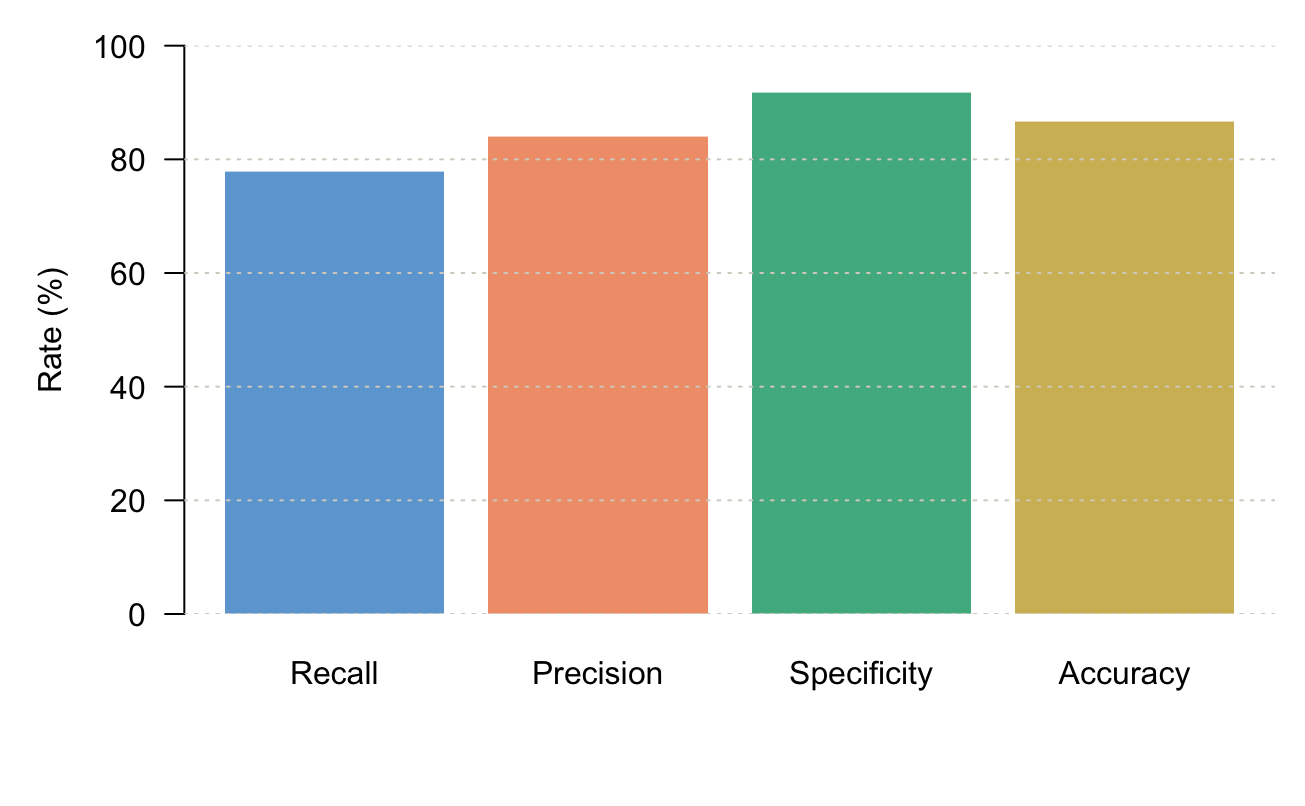
| TPR (Recall) | 77.78% | 108 | 4.00% | 73.78% | 81.78% | 69.78% | 85.78% |
| PPV (Precision) | 84.00% | 100 | 3.67% | 80.33% | 87.67% | 76.67% | 91.33% |
| TNR (Specificity) | 91.67% | 192 | 1.99% | 89.67% | 93.66% | 87.68% | 95.66% |
| NPV | 88.00% | 200 | 2.30% | 85.70% | 90.30% | 83.40% | 92.60% |
| Accuracy | 86.67% | 300 | 1.96% | 84.70% | 88.63% | 82.74% | 90.59% |
In this worked example, precision and recall are estimated on smaller denominators than accuracy, so their SD values are wider. That is expected: fewer effective trials imply greater rate uncertainty.
Rate profile figure
Interactive companion
Use the interactive tool at ED confusion matrix workbench to enter integer counts, calculate rates, and inspect the live distribution chart.
Class imbalance
When positive and negative observations are very unbalanced, the standard confusion matrix metrics behave differently and some become misleading.
Accuracy is unreliable under imbalance
A classifier that labels every observation negative achieves accuracy equal to the negative prevalence:
\[ \text{accuracy}_{\text{trivial}} = \frac{TN}{TP + FP + FN + TN} = \frac{N_-}{N}, \]
where \(N_-\) is the count of negative observations. If 95% of observations are negative, a null classifier reports 95% accuracy while having zero ability to detect positives.
Prevalence shifts PPV and NPV
PPV and NPV depend on the prevalence \(\pi = (TP + FN)/N\) through Bayes’ theorem even when sensitivity and specificity are fixed:
\[ \text{PPV} = \frac{\text{TPR} \cdot \pi}{\text{TPR} \cdot \pi + (1 - \text{TNR}) \cdot (1-\pi)}, \]
\[ \text{NPV} = \frac{\text{TNR} \cdot (1-\pi)}{\text{TNR} \cdot (1-\pi) + (1 - \text{TPR}) \cdot \pi}. \]
At low prevalence, PPV collapses even with high sensitivity and specificity. This is the false positive paradox common in rare-event screening: most positive calls are wrong.
Imbalance example
| Observed Predicted | Predicted + | Predicted - | Row total |
|---|---|---|---|
| + | 40 | 10 | 50 |
| - | 95 | 855 | 950 |
| Column total | 135 | 865 | 1000 |
| Metric | Balanced | Imbalanced |
|---|---|---|
| Prevalence | 28.0% | 4.0% |
| Accuracy | 86.7% | 89.5% |
| Recall (TPR) | 77.8% | 80.0% |
| Specificity (TNR) | 91.7% | 90.0% |
| Precision (PPV) | 84.0% | 29.6% |
| F1 | 80.8% | 43.2% |
| MCC | 0.707 | 0.446 |
Accuracy is nearly identical in both examples, which hides the degraded PPV in the imbalanced case.
Associated metrics under imbalance
- Recall (TPR) measures detection of actual positives and does not depend on \(N_-\).
- Precision (PPV) measures reliability of positive calls and is sensitive to the FP count.
- F1 score is the harmonic mean of precision and recall, penalising either being low.
- Balanced accuracy averages TPR and TNR, giving equal weight to both classes regardless of count:
\[ \text{balanced accuracy} = \frac{\text{TPR} + \text{TNR}}{2}. \]
- Matthews Correlation Coefficient (MCC) summarises all four cells in a single value between −1 and +1, robust to large imbalances:
\[ \text{MCC} = \frac{TP \cdot TN - FP \cdot FN}{\sqrt{(TP+FP)(TP+FN)(TN+FP)(TN+FN)}}. \]
An MCC of 0 corresponds to random guessing regardless of class balance; +1 indicates perfect prediction.
Planning under imbalance
When designing an experiment with rare positives:
- Set sample size against recall and precision targets, not accuracy.
- Report both PPV and NPV together with the observed prevalence so readers can recalibrate for different populations.
- Use stratified sampling or oversampling of the minority class to ensure the positive denominator is large enough for stable rate estimates.
References
- Chicco, D., & Jurman, G. (2020). The advantages of the Matthews correlation coefficient (MCC) over F1 score and accuracy in binary classification evaluation. BMC Genomics, 21(1), 6. https://doi.org/10.1186/s12864-019-6413-7
- Saito, T., & Rehmsmeier, M. (2015). The precision-recall plot is more informative than the ROC plot when evaluating binary classifiers on imbalanced datasets. PLOS ONE, 10(3), e0118432. https://doi.org/10.1371/journal.pone.0118432
- Vihinen, M. (2012). How to evaluate performance of prediction methods? Measures and their interpretation in variation effect analysis. BMC Genomics, 13(Suppl 4), S2. https://doi.org/10.1186/1471-2164-13-S4-S2